Introduction
Returns Based Style Analysis (RBSA) is a well known technique in portfolio optimisation that seeks to decompose an investment strategy (for example a mutual fund ) into underlying 'styles' such as Large Cap Growth, Small Cap Value etc.
Developed by Sharpe \([1]\), \([2]\), this technique represents the return series of an investment strategy over \(T\) time periods, \(\{R_t, \, t = 1, \ldots, T\}\), as a linear combination of \(n\) style factors \(F_i\), for example, passive market indices, with individual weightings, \(w_i\): \begin{align} R_t &= w_{1} F_{1t} + w_{2} F_{2t} + \cdots + w_{n} F_{nt} + \varepsilon_t, \qquad \qquad t = 1, \ldots, T \label{eq:1} \tag{I1} \\ \\ &= \mathbf{F_t} \cdot \mathbf{w} + \varepsilon_t \label{eq:2} \tag{I2} \end{align} where \(F_{it}\) is the return on the \(i^{th} \) style factor at time \(t\) in \(\eqref{eq:1}\)
and \(\mathbf{F_t}\), \(\mathbf{w}\) written in matrix notation in \(\eqref{eq:2}\) are below, \begin{equation} \mathbf{F_t} = \begin{bmatrix} F_{1t}, \, F_{2t}, \, \cdots, \, F_{nt} \end{bmatrix} \qquad \qquad \mathbf{w}= \begin{bmatrix} w_{1}, \, w_{2}, \, \cdots, \, w_{n} \end{bmatrix}^T \end{equation} (The RBSA model is therefore a special case of the more general linear factor model, \(R_t= \mathbf{F_t} \cdot \mathbf{w_t} + \varepsilon_t \), where the factor weights, \(w_{it}\), are time-invariant)
A benefit of this approach is that unlike fundamental analysis, which relies on the (often not readily available) actual holdings of the strategy to determine the style/asset class weighting, RBSA only requires the return series of the investment strategy and market indices which is relatively easily available for publically traded investments via common data vendors like Bloomberg and Morningstar.
Sharpe proposes choosing the weights \(w_i \) that minimises the variance of the non-factor returns \(\varepsilon_i\). In other words not seeking to minimise the distance between the strategy return stream \(R_{t}\) and the regression model \(\eqref{eq:2}\) but rather to minimise the variance of the distance so that the two time series look as close as possible to two equidistant lines. See picture below:
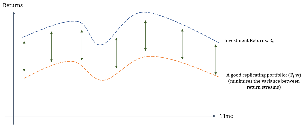
The (as close as possible) constant difference between the two return streams is interpreted by Sharpe as representing the manager's constant skill/contribution to the portfolio. This contribution can of course be negative.
The problem statement is therefore: Minimise the variance of \(\varepsilon_t \) by only varying the factor weights \(w_i \)
Mathematically: \begin{align} \min_{\mathbf{w} \in \mathbb{R}^n} \mbox{var}(\varepsilon_t) &= \mbox{var} (R_t - \mathbf{F_t} \cdot \mathbf{w}) \label{eq:3.0} \tag{I3}\\ \\ \mbox{subject to:} \quad \sum_{i=1}^{n} w_{i} &= 1 \label{eq:4} \tag{I4} \\ 0 \le w_i &\le 1, \quad \forall i \label{eq:5} \tag{I5} \end{align} Where the constraint \(\eqref{eq:5}\) describes the requirement of constructing a long only portfolio \(\mathbf{F_t}\) (i.e. weights cannot be negative) and without leverage (i.e. weights cannot be greater than \(1\))
Expanding \(\eqref{eq:3.0}\) and noting that, for a random variable \(X\), \(\mbox{var}(X) = \mathbb{E}[X^2] - (\mathbb{E}[X])^2 \): \begin{align} \mbox{var} (R_t - \mathbf{F_t} \cdot \mathbf{w}) &= \frac{1}{T} \sum_{t=1}^T(R_t - \mathbf{F_t} \cdot \mathbf{w})^2 - \left( \frac{1}{T}\sum_{t=1}^T(R_t - \mathbf{F_t} \cdot \mathbf{w}) \right)^2 \\ \\ &= \left( \frac{1}{T}\lVert \mathbf{R}\rVert ^2 - \frac{2}{T} \mathbf{R}^T \mathbf{F} \mathbf{w} + \frac{1}{T} \mathbf{w}^T \mathbf{F}^T \mathbf{F}\mathbf{w} \right ) - \left( \frac{e^T(\mathbf{R} - \mathbf{F} \mathbf{w})}{T} \right )^2 \\ \\ &= \frac{1}{T} \left(\lVert \mathbf{R}\rVert ^2 - 2 \mathbf{R}^T \mathbf{F} \mathbf{w} + \mathbf{w}^T \mathbf{F}^T \mathbf{F}\mathbf{w} \right ) - \frac{1}{T^2} \left( (e^T \mathbf{R})^2 -2 e^T \mathbf{R} e^T \mathbf{F}\mathbf{w} + \mathbf{w}^T \mathbf{F}^T e e^T \mathbf{F} \mathbf{w} \right ) \\ \\ &= \mathbf{w}^T \underbrace{\left( \frac{1}{T}\mathbf{F}^T \left( I - \frac{ee^T}{T} \right) \mathbf{F} \right )}_{\mathbf{D^{'}}} \mathbf{w} - \underbrace{2\left(\frac{\mathbf{R}^T\mathbf{F}}{T} - \frac{e^T \mathbf{R}}{T^2}e^T\mathbf{F}\right)}_\mathbf{d}\mathbf{w} + \underbrace{\left(\frac{\lVert \mathbf{R}\rVert ^2}{T} - \frac{(e^T \mathbf{R})^2}{T^2} \right)}_{c} \\ \end{align} where for simplicity in the above \begin{equation} \mathbf{R} = \begin{bmatrix} R_1\\ \vdots \\ R_T\\ \end{bmatrix} , \quad \mathbf{F} = \begin{pmatrix} F_{11} & \cdots & F_{n1}\\ \vdots & \ddots & \vdots\\ F_{1T} & \cdots & F_{nT}\\ \end{pmatrix} , \quad e = {\underbrace{\begin{bmatrix} 1, \, \cdots, \, 1 \end{bmatrix}}_{T}}^{T} \end{equation} Noting that the term \( c\) on the right-hand brace above is a constant independent of \(\mathbf{w} \) we have the problem stated as: \begin{align} \min_{\mathbf{w} \in \mathbb{R}^n} \mbox{var}(\varepsilon_t) &= \frac{1}{2} \mathbf{w}^T \! \cdot \! \mathbf{D} \! \cdot \! \mathbf{w} -\mathbf{d} \! \cdot \! \mathbf{w} \label{eq:6} \tag{I6} \end{align} subject to constraints \(\eqref{eq:4}\) and \(\eqref{eq:5}\)
where \begin{equation} \mathbf{D} = 2\mathbf{D^{'}} = \frac{2}{T}\mathbf{F}^T \left( I - \frac{ee^T}{T} \right) \mathbf{F} \quad \mbox{and} \quad \mathbf{d} = 2\left(\frac{\mathbf{R}^T\mathbf{F}}{T} - \frac{e^T \mathbf{R}}{T^2}e^T\mathbf{F}\right) \label{eq:7} \tag{I7} \end{equation}
Implementing in R:
Link to my GitHub repo: Returns-Based-Style-Analysis
So how do we go about using R to solve the optimisation problem represented in equation \(\eqref{eq:6}\)? As luck would have it R has a quadratic programming (QP) solver in the quadprog package to solve precisely this QP problem
Quoting directly from the description in the cran quadprog package documentation:
"This routine implements the dual method of Goldfarb and Idnani (1982, 1983) for solving quadratic programming problems of the form \begin{align} \min_{\mathbf{w} \in \mathbb{R}^n} \frac{1}{2} \mathbf{w}^T \! \cdot \! \mathbf{D} \! \cdot \! \mathbf{w} -\mathbf{d}^T \! \cdot \! \mathbf{w} \\ \\ \mbox{with the constraints:} \quad \mathbf{A}^T\mathbf{w} \ge \mathbf{b}_0 \label{eq:8} \tag{I8} \end{align} This is implemented in R by calling the QP-solver: \begin{equation} \mbox{solve.QP(Dmat}= \mathbf{D} \mbox{, dvec}= \mathbf{d} \mbox{, Amat}= \mathbf{A}, \mbox{bvec}= \mathbf{b}_0, m_{eq}=1) \end{equation} where \( m_{eq} \) specifies the first number of constraints in \(\eqref{eq:8}\) to be treated as equalities, with the remainder as inequalities."
The below steps through an example of how to construct the optimisation matrices, \( \mathbf{D}, \mathbf{d}, \mathbf{A}, \) and \(\mathbf{b_0}\) needed for a RBSA, given only the return streams of an investment strategy \(R_{t}\) and style factors \( \mathbf{F_t} \), and how this is implemented using quadprog.
This example uses a simulated return stream over \(T = 10 \) time periods with a choice of \(4\) underlying indicies
	#####################################
	# Title: Returns Based Style Analysis
	# Author: Thomas Handscomb
	#####################################

	#~~~~~~~~~~~~~~~~~~~~~~~~~~~~~~~~~~~~~~~~
	# Install packages and load into R session
	#install.packages("quadprog")
	#install.packages("matrix")

	library(quadprog)
	library(Matrix)

	#~~~~~~~~~~~~~~~~~~~~~~~~~~~~~~~~~~~~~~~~~~~~~~~~~~~~~~~~~
	# Specify the fund returns matrix over T = 10 time periods

	T=10
	R <- matrix(c(1.5, 1.6, 1.75, 1.70, 1.63, 1.59, 1.50, 1.59, 1.65, 1.70))

	# n = 4 Index returns over T=10 time periods
	n = 4

	# The n style factor return streams
	F1 <- c(0.76, 0.81, 0.89, 0.80, 0.81, 0.80, 0.79, 0.75, 0.69, 0.75)
	F2 <- c(0.93, 0.45, 0.76, 0.45, 0.54, 0.64, 0.74, 0.56, 0.59, 0.45)
	F3 <- c(0.15, 0.17, 0.21, 0.23, 0.26, 0.27, 0.28, 0.26, 0.23, 0.23)
	F4 <- c(0.20, 0.25, 0.32, 0.35, 0.32, 0.30, 0.25, 0.18, 0.10, 0.09)

	F <- as.matrix(cbind(F1, F2, F3, F4))
Define the optimisation matrices, \( \mathbf{D} \) and \( \mathbf{d} \). Recall the derivation of these in \(\eqref{eq:7}\)
	# Calculate the symmetric, positive definite matrix D
	e = matrix(1,T,1)

	M <- diag(T) - ((e %*% t(e))/T)
	M

	D <- (2/T)*t(F) %*% M %*% F

	# Check that D is symmetric, positive semi-definite
	D - (D+t(D))/2

	# Calculate the dvec
	d <- 2*(((1/T) * t(R) %*% F) - (1/(T^2))*(t(e) %*% R %*% t(e) %*% F))
The linear constraints \( A^T\mathbf{w} \ge \mathbf{b}_0 \) need to capture the contraints \(\eqref{eq:4}\) and \(\eqref{eq:5}\). This is achieved via
\begin{equation} A =
\begin{pmatrix}
1,1,0,0,0,-1,0,0,0 \\
1,0,1,0,0,0,-1,0,0 \\
1,0,0,1,0,0,0,-1,0 \\
1,0,0,0,1,0,0,0,-1 \\
\end{pmatrix}
\quad \mbox{and} \quad \mathbf{b}_0 =
\begin{pmatrix}
1,0,0,0,0,-1,-1,-1,-1 \\
\end{pmatrix}^T
\end{equation}
where the equality constraint \(\eqref{eq:4}\) is captured by the \( \mbox{solve.QP} \) parameter \( m_{eq}=1 \)
	# Build up the constraint matrices:
	A <- t(rbind(rep(1,n), diag(n), -diag(n)))
	A

	# Define the constraint coefficient column vector b0
	b0 <- matrix(c(1, rep(0,n), rep(-1,n)))
	b0
Call the QP Solver, extract solution coefficients and construct the optimial solution as \( \mathbf{F} \cdot \mathbf{w} \)
	# Call the QP solver, note input the transpose of d
	sol <- solve.QP(Dmat = D, dvec = t(d), Amat = A, bvec = b0, meq = 1)

	# The solution gives the vector w comprised of optimal weights
	wvec = as.matrix(sol$solution)

	#> wvec
		#[,1]
	#[1,] 0.6679001
	#[2,] 0.0000000
	#[3,] 0.3320999
	#[4,] 0.0000000

	# Double check that the sum of the w_i coefficients = 1
	sum(wvec)
	#> sum(wvec)
	#[1] 1

	# Once the weight matrix has been constructed, the optimal solution can then be constructed
	opsol <- F %*% wvec
	opsol

	# Calculate the fit of the optimal solution
	# recall the optimisation model is minimising var(R-F*wvec)
	var(R-opsol) #0.006430116
The plot of both the investment and optimal solution returns gives some suggestion that the optimiser has indeed minimised the variance between the two return streams
	# View a plot of the return stream and the optimal solution
	plot(R, ylim = c(0.0, 2.50), type = 'b'
	 , main="Return stream vs. Optimal solution"
	 , xlab="Time"
	 , ylab="Return")
	points(opsol, col = 'blue', type = 'b')
	legend("topleft", legend=c("Investment", "Optimal Solution")
	   , col=c("black", "blue")
	   , lty=c(1,1))
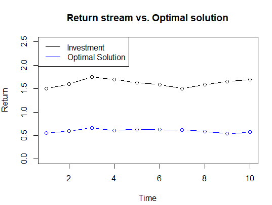 Compare this plot to Figure 1
 As a check to the optimality, let's see if we can find a better solution at random, i.e. a random choice of \( \mathbf{w} \) that achieves a lower \( \mbox{var} (R_t - \mathbf{F_t} \cdot \mathbf{w}) \) than the \( 0.006430116 \) of the optimal solution
	#~~~~~~~~~~~~~~~~~~~~~~~~~~~~~~~~~~~~~~~~~~~~~~~~~~~~~~~~~~~~~~~~~~~~~~~~~~~
	# Try 10000 random solutions to check that you can't achieve a lower variance

	# First create solution data frame with first row as the QP solved optimal solution
	df_solutions = data.frame("Solution_ID" = character(0), "Variance" = numeric(0))
	df_solutions = rbind(df_solutions, c(as.character("Optimal"), as.numeric(var(R-opsol))))
	colnames(df_solutions) <- c("Solution_Id", "Variance")
	#head(df_solutions)

	# Then create 10000 random choices of weights that sum to 1 and corresponding random solutions
	for (i in 1:10000){
	  # Define random weights
	  R4 <- runif(4)
	  R4 <- R4/sum(R4)
	  rancoef1 = R4[1]
	  rancoef2 = R4[2]
	  rancoef3 = R4[3]
	  rancoef4 = R4[4]
	  random_wvec = as.matrix(c(rancoef1, rancoef2, rancoef3, rancoef4))

	  # Construct the solution corresponding to the random weights
	  randomsol = F %*% random_wvec

	  # Create a temporary dataframe containing the iteration solution
	  df_temp = data.frame("Solution_ID" = character(0), "Variance" = numeric(0))
	  df_temp = rbind(df_temp, c(paste0("RanSol_",i), var(R-randomsol)))
	  colnames(df_temp) <- c("Solution_Id", "Variance")

	  # Append iteration solution to the total solution dataframe
	  df_solutions = rbind(df_solutions, df_temp)
	}
	# The rbind has created Variance as a factor...
	sapply(df_solutions, class)
	#...so convert back to numeric
	df_solutions$Variance = as.numeric(paste(df_solutions$Variance))
	sapply(df_solutions, class)

	# Sort the solution dataframe by descending Variance, show the lowest 10 only
	head(df_solutions[order(df_solutions$Variance),], 10)

		#Solution_Id    Variance
	#1        Optimal 0.006430116
	#8607 RanSol_8606 0.006632959
	#4117 RanSol_4116 0.006643589
	#509   RanSol_508 0.006652932
	#8542 RanSol_8541 0.006659689
	#6736 RanSol_6735 0.006747747
	#7805 RanSol_7804 0.006753655
	#4066 RanSol_4065 0.006755018
	#9213 RanSol_9212 0.006757928
	#7053 RanSol_7052 0.006819245

	# Optimal solution is still the best!
References:
- \([1]\) W. F. Sharpe. Determining a fund’s effective asset mix. Investment Management Review, pages 59–69, December 1988.
- \([2]\) W. F. Sharpe. Asset allocation: Management style and performance measurement. Journal of Portfolio Management, pages 7–19, Winter 1992.